VARLiNGAM
Model
VARLiNGAM [2] is an extension of the basic LiNGAM model [1] to time series cases. It combines the basic LiNGAM model with the classic vector autoregressive models (VAR). It enables analyzing both lagged and contemporaneous (instantaneous) causal relations, whereas the classic VAR only analyzes lagged causal relations. This VARLiNGAM makes the following assumptions similarly to the basic LiNGAM model [1]:
Linearity
Non-Gaussian continuous error variables (except at most one)
Acyclicity of contemporaneous causal relations
No hidden common causes
Denote observed variables at time point \({t}\) by \({x}_{i}(t)\) and error variables by \({e}_{i}(t)\). Collect them in vectors \({x}(t)\) and \({e}(t)\), respectivelly. Further, denote by matrices \({B}_{\tau}\) adjacency matrices with time lag \({\tau}\).
Due to the acyclicity assumption of contemporaneous causal relations, the coefficient matrix \({B}_{0}\) can be permuted to be strictly lower-triangular by a simultaneous row and column permutation. The error variables \({e}_{i}(t)\) are independent due to the assumption of no hidden common causes.
Then, mathematically, the model for observed variable vector \({x}(t)\) is written as
$$ x(t) = \sum_{ \tau = 0}^k B_{ \tau } x(t - \tau) + e(t).$$
Example applications are found here, especially in Section. Economics/Finance/Marketing. For example, [3] uses the VARLiNGAM model to to study the processes of firm growth and firm performance using microeconomic data and to analyse the effects of monetary policy using macroeconomic data.
References
Import and settings
In this example, we need to import numpy, pandas, and
graphviz in addition to lingam.
import numpy as np
import pandas as pd
import graphviz
import lingam
from lingam.utils import make_dot, print_causal_directions, print_dagc

print([np.__version__, pd.__version__, graphviz.__version__, lingam.__version__])

np.set_printoptions(precision=3, suppress=True)
np.random.seed(0)
['1.24.4', '2.0.3', '0.20.1', '1.8.3']
Test data
We create test data consisting of 5 variables.
B0 = [
    [0,-0.12,0,0,0],
    [0,0,0,0,0],
    [-0.41,0.01,0,-0.02,0],
    [0.04,-0.22,0,0,0],
    [0.15,0,-0.03,0,0],
]
B1 = [
    [-0.32,0,0.12,0.32,0],
    [0,-0.35,-0.1,-0.46,0.4],
    [0,0,0.37,0,0.46],
    [-0.38,-0.1,-0.24,0,-0.13],
    [0,0,0,0,0],
]
causal_order = [1, 0, 3, 2, 4]

# data generated from B0 and B1
X = pd.read_csv('data/sample_data_var_lingam.csv')
Causal Discovery
To run causal discovery, we create a VARLiNGAM object and call the fit() method.
model = lingam.VARLiNGAM()
model.fit(X)
<lingam.var_lingam.VARLiNGAM at 0x7fc1a642d970>
Using the causal_order_ properties, we can see the causal ordering as a result of the causal discovery.
model.causal_order_
[1, 0, 3, 2, 4]
Also, using the adjacency_matrices_ properties, we can see the adjacency matrix as a result of the causal discovery.
# B0
model.adjacency_matrices_[0]
array([[ 0.   , -0.136,  0.   ,  0.   ,  0.   ],
       [ 0.   ,  0.   ,  0.   ,  0.   ,  0.   ],
       [-0.484,  0.   ,  0.   ,  0.   ,  0.   ],
       [ 0.075, -0.21 ,  0.   ,  0.   ,  0.   ],
       [ 0.168,  0.   ,  0.   ,  0.   ,  0.   ]])
# B1
model.adjacency_matrices_[1]
array([[-0.358,  0.   ,  0.073,  0.302,  0.   ],
       [ 0.   , -0.338, -0.154, -0.335,  0.423],
       [ 0.   ,  0.   ,  0.424,  0.112,  0.493],
       [-0.386, -0.1  , -0.266,  0.   , -0.159],
       [ 0.   ,  0.   ,  0.   ,  0.   ,  0.   ]])
model.residuals_
array([[-0.308,  0.911, -1.152, -1.159,  0.179],
       [ 1.364,  1.713, -1.389, -0.265, -0.192],
       [-0.861,  0.249,  0.479, -1.557, -0.462],
       ...,
       [-1.202,  1.819,  0.99 , -0.855, -0.127],
       [-0.133,  1.23 , -0.445, -0.753,  1.096],
       [-0.069,  0.558,  0.21 , -0.863, -0.189]])
Using DirectLiNGAM for the residuals_ properties, we can
calculate B0 matrix.
dlingam = lingam.DirectLiNGAM()
dlingam.fit(model.residuals_)
dlingam.adjacency_matrix_
array([[ 0.   , -0.144,  0.   ,  0.   ,  0.   ],
       [ 0.   ,  0.   ,  0.   ,  0.   ,  0.   ],
       [-0.456,  0.   ,  0.   ,  0.   ,  0.   ],
       [ 0.   , -0.22 ,  0.   ,  0.   ,  0.   ],
       [ 0.157,  0.   ,  0.   ,  0.   ,  0.   ]])
We can draw a causal graph by utility funciton.
labels = ['x0(t)', 'x1(t)', 'x2(t)', 'x3(t)', 'x4(t)', 'x0(t-1)', 'x1(t-1)', 'x2(t-1)', 'x3(t-1)', 'x4(t-1)']
make_dot(np.hstack(model.adjacency_matrices_), ignore_shape=True, lower_limit=0.05, labels=labels)

Independence between error variables
To check if the LiNGAM assumption is broken, we can get p-values of independence between error variables. The value in the i-th row and j-th column of the obtained matrix shows the p-value of the independence of the error variables \(e_i\) and \(e_j\).
p_values = model.get_error_independence_p_values()
print(p_values)
[[0.    0.127 0.104 0.042 0.746]
 [0.127 0.    0.086 0.874 0.739]
 [0.104 0.086 0.    0.404 0.136]
 [0.042 0.874 0.404 0.    0.763]
 [0.746 0.739 0.136 0.763 0.   ]]
Bootstrap
Bootstrapping
We call bootstrap() method instead of fit(). Here, the second argument specifies the number of bootstrap sampling.
model = lingam.VARLiNGAM()
result = model.bootstrap(X, n_sampling=100)
Causal Directions
Since BootstrapResult object is returned, we can get the ranking of the causal directions extracted by get_causal_direction_counts() method. In the following sample code, n_directions option is limited to the causal directions of the top 8 rankings, and min_causal_effect option is limited to causal directions with a coefficient of 0.3 or more.
cdc = result.get_causal_direction_counts(n_directions=8, min_causal_effect=0.3, split_by_causal_effect_sign=True)
We can check the result by utility function.
print_causal_directions(cdc, 100, labels=labels)
x2(t) <--- x4(t-1) (b>0) (100.0%)
x2(t) <--- x2(t-1) (b>0) (100.0%)
x0(t) <--- x0(t-1) (b<0) (95.0%)
x1(t) <--- x1(t-1) (b<0) (86.0%)
x1(t) <--- x4(t-1) (b>0) (85.0%)
x3(t) <--- x0(t-1) (b<0) (78.0%)
x2(t) <--- x4(t) (b<0) (60.0%)
x0(t) <--- x3(t-1) (b>0) (48.0%)
Directed Acyclic Graphs
Also, using the get_directed_acyclic_graph_counts() method, we can get the ranking of the DAGs extracted. In the following sample code, n_dags option is limited to the dags of the top 3 rankings, and min_causal_effect option is limited to causal directions with a coefficient of 0.2 or more.
dagc = result.get_directed_acyclic_graph_counts(n_dags=3, min_causal_effect=0.2, split_by_causal_effect_sign=True)
We can check the result by utility function.
print_dagc(dagc, 100, labels=labels)
DAG[0]: 5.0%
    x0(t) <--- x0(t-1) (b<0)
    x0(t) <--- x3(t-1) (b>0)
    x1(t) <--- x0(t) (b<0)
    x1(t) <--- x0(t-1) (b<0)
    x1(t) <--- x1(t-1) (b<0)
    x1(t) <--- x4(t-1) (b>0)
    x2(t) <--- x0(t) (b<0)
    x2(t) <--- x4(t) (b<0)
    x2(t) <--- x2(t-1) (b>0)
    x2(t) <--- x4(t-1) (b>0)
    x3(t) <--- x0(t) (b>0)
    x3(t) <--- x0(t-1) (b<0)
    x3(t) <--- x2(t-1) (b<0)
    x3(t) <--- x4(t-1) (b<0)
DAG[1]: 5.0%
    x0(t) <--- x0(t-1) (b<0)
    x0(t) <--- x3(t-1) (b>0)
    x1(t) <--- x0(t) (b<0)
    x1(t) <--- x2(t) (b>0)
    x1(t) <--- x0(t-1) (b<0)
    x1(t) <--- x1(t-1) (b<0)
    x1(t) <--- x4(t-1) (b>0)
    x2(t) <--- x0(t) (b<0)
    x2(t) <--- x4(t) (b<0)
    x2(t) <--- x2(t-1) (b>0)
    x2(t) <--- x4(t-1) (b>0)
    x3(t) <--- x0(t) (b>0)
    x3(t) <--- x0(t-1) (b<0)
    x3(t) <--- x2(t-1) (b<0)
DAG[2]: 5.0%
    x0(t) <--- x0(t-1) (b<0)
    x0(t) <--- x3(t-1) (b>0)
    x1(t) <--- x1(t-1) (b<0)
    x1(t) <--- x3(t-1) (b<0)
    x1(t) <--- x4(t-1) (b>0)
    x2(t) <--- x1(t) (b>0)
    x2(t) <--- x3(t) (b>0)
    x2(t) <--- x0(t-1) (b>0)
    x2(t) <--- x2(t-1) (b>0)
    x2(t) <--- x4(t-1) (b>0)
    x3(t) <--- x1(t) (b<0)
    x3(t) <--- x0(t-1) (b<0)
    x3(t) <--- x2(t-1) (b<0)
Probability
Using the get_probabilities() method, we can get the probability of bootstrapping.
prob = result.get_probabilities(min_causal_effect=0.1)
print('Probability of B0:\n', prob[0])
print('Probability of B1:\n', prob[1])
Probability of B0:
 [[0.   0.6  0.04 0.06 0.14]
 [0.39 0.   0.25 0.18 0.16]
 [0.65 0.68 0.   0.67 0.84]
 [0.51 0.6  0.07 0.   0.66]
 [0.35 0.28 0.01 0.09 0.  ]]
Probability of B1:
 [[1.   0.   0.3  1.   0.02]
 [0.56 1.   0.94 0.67 1.  ]
 [0.8  0.02 1.   0.25 1.  ]
 [1.   0.24 1.   0.08 1.  ]
 [0.02 0.   0.03 0.07 0.  ]]
Total Causal Effects
Using the get_causal_effects() method, we can get the list of total
causal effect. The total causal effects we can get are dictionary type
variable. We can display the list nicely by assigning it to
pandas.DataFrame. Also, we have replaced the variable index with a label
below.
causal_effects = result.get_total_causal_effects(min_causal_effect=0.01)
df = pd.DataFrame(causal_effects)

df['from'] = df['from'].apply(lambda x : labels[x])
df['to'] = df['to'].apply(lambda x : labels[x])
df
| from | to | effect | probability | |
|---|---|---|---|---|
| 0 | x0(t-1) | x2(t) | 0.181032 | 1.00 |
| 1 | x2(t-1) | x2(t) | 0.388777 | 1.00 |
| 2 | x4(t-1) | x1(t) | 0.427308 | 1.00 |
| 3 | x1(t-1) | x1(t) | -0.338691 | 1.00 |
| 4 | x0(t-1) | x3(t) | -0.397439 | 1.00 |
| 5 | x3(t-1) | x0(t) | 0.345461 | 1.00 |
| 6 | x4(t-1) | x2(t) | 0.501859 | 1.00 |
| 7 | x4(t-1) | x3(t) | -0.253700 | 1.00 |
| 8 | x0(t-1) | x0(t) | -0.357296 | 1.00 |
| 9 | x2(t-1) | x3(t) | -0.222886 | 1.00 |
| 10 | x3(t-1) | x3(t) | 0.101008 | 1.00 |
| 11 | x3(t-1) | x1(t) | -0.315462 | 0.99 |
| 12 | x2(t-1) | x0(t) | 0.090369 | 0.99 |
| 13 | x2(t-1) | x1(t) | -0.172693 | 0.98 |
| 14 | x1(t-1) | x2(t) | -0.063602 | 0.89 |
| 15 | x4(t) | x2(t) | -0.449165 | 0.89 |
| 16 | x3(t-1) | x2(t) | -0.079600 | 0.89 |
| 17 | x0(t) | x2(t) | -0.280635 | 0.83 |
| 18 | x1(t-1) | x0(t) | 0.057164 | 0.82 |
| 19 | x4(t-1) | x0(t) | -0.050805 | 0.79 |
| 20 | x4(t) | x3(t) | -0.151835 | 0.76 |
| 21 | x1(t) | x2(t) | 0.211957 | 0.75 |
| 22 | x1(t-1) | x3(t) | -0.021313 | 0.75 |
| 23 | x3(t) | x2(t) | 0.248101 | 0.66 |
| 24 | x0(t) | x3(t) | 0.259859 | 0.64 |
| 25 | x3(t-1) | x4(t) | 0.061849 | 0.62 |
| 26 | x1(t) | x3(t) | -0.218490 | 0.62 |
| 27 | x1(t) | x0(t) | -0.199704 | 0.61 |
| 28 | x1(t) | x4(t) | -0.104466 | 0.56 |
| 29 | x0(t-1) | x1(t) | -0.119971 | 0.53 |
| 30 | x2(t-1) | x4(t) | 0.017608 | 0.50 |
| 31 | x4(t-1) | x4(t) | -0.041991 | 0.47 |
| 32 | x1(t-1) | x4(t) | 0.029382 | 0.42 |
| 33 | x0(t-1) | x4(t) | -0.055934 | 0.42 |
| 34 | x4(t) | x1(t) | -0.063677 | 0.42 |
| 35 | x4(t) | x0(t) | -0.066867 | 0.40 |
| 36 | x0(t) | x1(t) | -0.719255 | 0.39 |
| 37 | x0(t) | x4(t) | 0.174717 | 0.37 |
| 38 | x2(t) | x1(t) | 0.212699 | 0.25 |
| 39 | x3(t) | x1(t) | -0.308596 | 0.20 |
| 40 | x2(t) | x3(t) | -0.084192 | 0.18 |
| 41 | x3(t) | x0(t) | 0.154238 | 0.11 |
| 42 | x3(t) | x4(t) | -0.205918 | 0.10 |
| 43 | x2(t) | x0(t) | -0.217316 | 0.06 |
| 44 | x2(t) | x4(t) | -0.093614 | 0.03 |
We can easily perform sorting operations with pandas.DataFrame.
df.sort_values('effect', ascending=False).head()
| from | to | effect | probability | |
|---|---|---|---|---|
| 6 | x4(t-1) | x2(t) | 0.501859 | 1.00 |
| 2 | x4(t-1) | x1(t) | 0.427308 | 1.00 |
| 1 | x2(t-1) | x2(t) | 0.388777 | 1.00 |
| 5 | x3(t-1) | x0(t) | 0.345461 | 1.00 |
| 24 | x0(t) | x3(t) | 0.259859 | 0.64 |
And with pandas.DataFrame, we can easily filter by keywords. The following code extracts the causal direction towards x1(t).
df[df['to']=='x1(t)'].head()
| from | to | effect | probability | |
|---|---|---|---|---|
| 2 | x4(t-1) | x1(t) | 0.427308 | 1.00 |
| 3 | x1(t-1) | x1(t) | -0.338691 | 1.00 |
| 11 | x3(t-1) | x1(t) | -0.315462 | 0.99 |
| 13 | x2(t-1) | x1(t) | -0.172693 | 0.98 |
| 29 | x0(t-1) | x1(t) | -0.119971 | 0.53 |
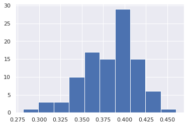
Because it holds the raw data of the causal effect (the original data for calculating the median), it is possible to draw a histogram of the values of the causal effect, as shown below.
import matplotlib.pyplot as plt
import seaborn as sns
sns.set()
%matplotlib inline

from_index = 7 # index of x2(t-1). (index:2)+(n_features:5)*(lag:1) = 7
to_index = 2 # index of x2(t). (index:2)+(n_features:5)*(lag:0) = 2
plt.hist(result.total_effects_[:, to_index, from_index])