Longitudinal LiNGAM
Model
This method [2] performs causal discovery on “paired” samples based on longitudinal data that collects samples over time. Their algorithm can analyze causal structures, including topological causal orders, that may change over time. Similarly to the basic LiNGAM model [1], this method makes the following assumptions:
Linearity
Non-Gaussian continuous error variables (except at most one)
Acyclicity
No hidden common causes
Denote observed variables and error variables of \({m}\)-the sample at time point \({m}\) by \({x}_{i}^{m}(t)\) and \({e}_{i}^{m}(t)\). Collect them from variables in vectors \({x}^{m}(t)\) and \({e}^{m}(t)\). Further, collect them from samples in matrices \({X}(t)\) and \({E}(t)\). Further, denote by \({B}(t,t-\tau)\) adjacency matrices with time lag \(\tau\).
Due to the assumptions of acyclicity, the adjacency matrix \({B}(t,t)\) can be permuted to be strictly lower-triangular by a simultaneous row and column permutation. The error variables \({e}_{i}^{m}(t)\) are independent due to the assumption of no hidden common causes.
Then, mathematically, the model for observed variable matrix \({X}(t)\) is written as
$$ X(t) = \sum_{ \tau = 0}^k B (t, t-\tau) X(t - \tau) + E(t).$$
References
Import and settings
In this example, we need to import numpy, pandas, and
graphviz in addition to lingam.
import numpy as np
import pandas as pd
import matplotlib.pyplot as plt
import graphviz
import lingam
from lingam.utils import print_causal_directions, print_dagc, make_dot

import warnings
warnings.filterwarnings('ignore')

print([np.__version__, pd.__version__, graphviz.__version__, lingam.__version__])

np.set_printoptions(precision=3, suppress=True)
np.random.seed(0)
['1.24.4', '2.0.3', '0.20.1', '1.8.3']
Test data
We create test data consisting of 5 variables. The causal model at each timepoint is as follows.
# setting
n_features = 5
n_samples = 200
n_lags = 1
n_timepoints = 3

causal_orders = []
B_t_true = np.empty((n_timepoints, n_features, n_features))
B_tau_true = np.empty((n_timepoints, n_lags, n_features, n_features))
X_t = np.empty((n_timepoints, n_samples, n_features))
# B(0,0)
B_t_true[0] = np.array([[0.0, 0.5,-0.3, 0.0, 0.0],
                        [0.0, 0.0,-0.3, 0.4, 0.0],
                        [0.0, 0.0, 0.0, 0.3, 0.0],
                        [0.0, 0.0, 0.0, 0.0, 0.0],
                        [0.1,-0.7, 0.0, 0.0, 0.0]])
causal_orders.append([3, 2, 1, 0, 4])
make_dot(B_t_true[0], labels=[f'x{i}(0)' for i in range(5)])

# B(1,1)
B_t_true[1] = np.array([[0.0, 0.2,-0.1, 0.0,-0.5],
                        [0.0, 0.0, 0.0, 0.4, 0.0],
                        [0.0, 0.3, 0.0, 0.0, 0.0],
                        [0.0, 0.0, 0.0, 0.0, 0.0],
                        [0.0,-0.4, 0.0, 0.0, 0.0]])
causal_orders.append([3, 1, 2, 4, 0])
make_dot(B_t_true[1], labels=[f'x{i}(1)' for i in range(5)])

# B(2,2)
B_t_true[2] = np.array([[0.0, 0.0, 0.0, 0.0, 0.0],
                        [0.0, 0.0,-0.7, 0.0, 0.5],
                        [0.2, 0.0, 0.0, 0.0, 0.0],
                        [0.0, 0.0,-0.4, 0.0, 0.0],
                        [0.3, 0.0, 0.0, 0.0, 0.0]])
causal_orders.append([0, 2, 4, 3, 1])
make_dot(B_t_true[2], labels=[f'x{i}(2)' for i in range(5)])

# create B(t,t-τ) and X
for t in range(n_timepoints):
    # external influence
    expon = 0.1
    ext = np.empty((n_features, n_samples))
    for i in range(n_features):
        ext[i, :] = np.random.normal(size=(1, n_samples));
        ext[i, :] = np.multiply(np.sign(ext[i, :]), abs(ext[i, :]) ** expon);
        ext[i, :] = ext[i, :] - np.mean(ext[i, :]);
        ext[i, :] = ext[i, :] / np.std(ext[i, :]);

    # create B(t,t-τ)
    for tau in range(n_lags):
        value = np.random.uniform(low=0.01, high=0.5, size=(n_features, n_features))
        sign = np.random.choice([-1, 1], size=(n_features, n_features))
        B_tau_true[t, tau] = np.multiply(value, sign)

    # create X(t)
    X = np.zeros((n_features, n_samples))
    for co in causal_orders[t]:
        X[co] = np.dot(B_t_true[t][co, :], X) + ext[co]
        if t > 0:
            for tau in range(n_lags):
                X[co] = X[co] + np.dot(B_tau_true[t, tau][co, :], X_t[t-(tau+1)].T)

    X_t[t] = X.T
Causal Discovery
To run causal discovery, we create a LongitudinalLiNGAM object by specifying the n_lags parameter. Then, we call the fit() method.
model = lingam.LongitudinalLiNGAM(n_lags=n_lags)
model = model.fit(X_t)
Using the causal_orders_ property, we can see the causal ordering in time-points as a result of the causal discovery. All elements are nan because the causal order of B(t,t) at t=0 is not calculated. So access to the time points above t=1.
print(model.causal_orders_[0]) # nan at t=0
print(model.causal_orders_[1])
print(model.causal_orders_[2])
[nan, nan, nan, nan, nan]
[3, 1, 2, 4, 0]
[0, 4, 2, 3, 1]
Also, using the adjacency_matrices_ property, we can see the adjacency matrix as a result of the causal discovery. As with the causal order, all elements are nan because the B(t,t) and B(t,t-τ) at t=0 is not calculated. So access to the time points above t=1. Also, if we run causal discovery with n_lags=2, B(t,t-τ) at t=1 is also not computed, so all the elements are nan.
t = 0 # nan at t=0
print('B(0,0):')
print(model.adjacency_matrices_[t, 0])
print('B(0,-1):')
print(model.adjacency_matrices_[t, 1])

t = 1
print('B(1,1):')
print(model.adjacency_matrices_[t, 0])
print('B(1,0):')
print(model.adjacency_matrices_[t, 1])

t = 2
print('B(2,2):')
print(model.adjacency_matrices_[t, 0])
print('B(2,1):')
print(model.adjacency_matrices_[t, 1])
B(0,0):
[[nan nan nan nan nan]
 [nan nan nan nan nan]
 [nan nan nan nan nan]
 [nan nan nan nan nan]
 [nan nan nan nan nan]]
B(0,-1):
[[nan nan nan nan nan]
 [nan nan nan nan nan]
 [nan nan nan nan nan]
 [nan nan nan nan nan]
 [nan nan nan nan nan]]
B(1,1):
[[ 0.     0.     0.     0.    -0.611]
 [ 0.     0.     0.     0.398  0.   ]
 [ 0.     0.328  0.     0.     0.   ]
 [ 0.     0.     0.     0.     0.   ]
 [ 0.    -0.338  0.     0.     0.   ]]
B(1,0):
[[ 0.029  0.064 -0.27   0.065 -0.18 ]
 [ 0.139 -0.211 -0.43   0.558  0.051]
 [-0.181  0.178  0.466  0.214  0.079]
 [ 0.384 -0.083 -0.495 -0.072 -0.323]
 [-0.174 -0.383 -0.274 -0.275  0.457]]
B(2,2):
[[ 0.     0.     0.     0.     0.   ]
 [ 0.     0.    -0.696  0.     0.487]
 [ 0.231  0.     0.     0.     0.   ]
 [ 0.     0.    -0.409  0.     0.   ]
 [ 0.25   0.     0.     0.     0.   ]]
B(2,1):
[[ 0.194  0.2    0.031 -0.473 -0.002]
 [-0.376 -0.038  0.16   0.261  0.102]
 [ 0.117  0.266 -0.05   0.523 -0.019]
 [ 0.249 -0.448  0.473 -0.001 -0.177]
 [-0.177  0.309 -0.112  0.295 -0.273]]
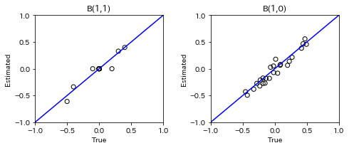
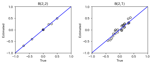
for t in range(1, n_timepoints):
    B_t, B_tau = model.adjacency_matrices_[t]
    plt.figure(figsize=(7, 3))

    plt.subplot(1,2,1)
    plt.plot([-1, 1],[-1, 1], marker="", color="blue", label="support")
    plt.scatter(B_t_true[t], B_t, facecolors='none', edgecolors='black')
    plt.xlim(-1, 1)
    plt.ylim(-1, 1)
    plt.xlabel('True')
    plt.ylabel('Estimated')
    plt.title(f'B({t},{t})')

    plt.subplot(1,2,2)
    plt.plot([-1, 1],[-1, 1], marker="", color="blue", label="support")
    plt.scatter(B_tau_true[t], B_tau, facecolors='none', edgecolors='black')
    plt.xlim(-1, 1)
    plt.ylim(-1, 1)
    plt.xlabel('True')
    plt.ylabel('Estimated')
    plt.title(f'B({t},{t-1})')

    plt.tight_layout()
    plt.show()
Independence between error variables
To check if the LiNGAM assumption is broken, we can get p-values of independence between error variables. The value in the i-th row and j-th column of the obtained matrix shows the p-value of the independence of the error variables \(e_i\) and \(e_j\).
p_values_list = model.get_error_independence_p_values()
t = 1
print(p_values_list[t])
[[0.    0.026 0.064 0.289 0.051]
 [0.026 0.    0.363 0.821 0.581]
 [0.064 0.363 0.    0.067 0.098]
 [0.289 0.821 0.067 0.    0.059]
 [0.051 0.581 0.098 0.059 0.   ]]
t = 2
print(p_values_list[2])
[[0.    0.715 0.719 0.593 0.564]
 [0.715 0.    0.78  0.7   0.504]
 [0.719 0.78  0.    0.532 0.591]
 [0.593 0.7   0.532 0.    0.401]
 [0.564 0.504 0.591 0.401 0.   ]]
Bootstrapping
We call bootstrap() method instead of fit(). Here, the second argument specifies the number of bootstrap sampling.
model = lingam.LongitudinalLiNGAM()
result = model.bootstrap(X_t, n_sampling=100)
Causal Directions
Since LongitudinalBootstrapResult object is returned, we can get the ranking of the causal directions extracted by get_causal_direction_counts() method. In the following sample code, n_directions option is limited to the causal directions of the top 8 rankings, and min_causal_effect option is limited to causal directions with a coefficient of 0.01 or more.
cdc_list = result.get_causal_direction_counts(n_directions=12, min_causal_effect=0.01, split_by_causal_effect_sign=True)
t = 1
labels = [f'x{i}({u})' for u in [t, t-1] for i in range(5)]
print_causal_directions(cdc_list[t], 100, labels=labels)
x2(1) <--- x0(0) (b<0) (100.0%)
x4(1) <--- x1(0) (b<0) (100.0%)
x4(1) <--- x1(1) (b<0) (100.0%)
x3(1) <--- x4(0) (b<0) (100.0%)
x3(1) <--- x2(0) (b<0) (100.0%)
x3(1) <--- x0(0) (b>0) (100.0%)
x2(1) <--- x2(0) (b>0) (100.0%)
x1(1) <--- x3(0) (b>0) (100.0%)
x1(1) <--- x2(0) (b<0) (100.0%)
x1(1) <--- x3(1) (b>0) (100.0%)
x4(1) <--- x4(0) (b>0) (100.0%)
x0(1) <--- x4(1) (b<0) (100.0%)
t = 2
labels = [f'x{i}({u})' for u in [t, t-1] for i in range(5)]
print_causal_directions(cdc_list[t], 100, labels=labels)
x0(2) <--- x0(1) (b>0) (100.0%)
x4(2) <--- x1(1) (b>0) (100.0%)
x4(2) <--- x0(1) (b<0) (100.0%)
x3(2) <--- x2(1) (b>0) (100.0%)
x3(2) <--- x1(1) (b<0) (100.0%)
x3(2) <--- x0(1) (b>0) (100.0%)
x3(2) <--- x2(2) (b<0) (100.0%)
x2(2) <--- x3(1) (b>0) (100.0%)
x2(2) <--- x1(1) (b>0) (100.0%)
x4(2) <--- x3(1) (b>0) (100.0%)
x1(2) <--- x3(1) (b>0) (100.0%)
x1(2) <--- x2(1) (b>0) (100.0%)
Directed Acyclic Graphs
Also, using the get_directed_acyclic_graph_counts() method, we can get the ranking of the DAGs extracted. In the following sample code, n_dags option is limited to the dags of the top 3 rankings, and min_causal_effect option is limited to causal directions with a coefficient of 0.01 or more.
dagc_list = result.get_directed_acyclic_graph_counts(n_dags=3, min_causal_effect=0.01, split_by_causal_effect_sign=True)
t = 1
labels = [f'x{i}({u})' for u in [t, t-1] for i in range(5)]
print_dagc(dagc_list[t], 100, labels=labels)
DAG[0]: 2.0%
    x0(1) <--- x1(1) (b>0)
    x0(1) <--- x3(1) (b>0)
    x0(1) <--- x4(1) (b<0)
    x0(1) <--- x0(0) (b<0)
    x0(1) <--- x1(0) (b>0)
    x0(1) <--- x2(0) (b<0)
    x0(1) <--- x3(0) (b<0)
    x0(1) <--- x4(0) (b<0)
    x1(1) <--- x3(1) (b>0)
    x1(1) <--- x0(0) (b>0)
    x1(1) <--- x1(0) (b<0)
    x1(1) <--- x2(0) (b<0)
    x1(1) <--- x3(0) (b>0)
    x1(1) <--- x4(0) (b>0)
    x2(1) <--- x1(1) (b>0)
    x2(1) <--- x0(0) (b<0)
    x2(1) <--- x1(0) (b>0)
    x2(1) <--- x2(0) (b>0)
    x2(1) <--- x3(0) (b>0)
    x2(1) <--- x4(0) (b>0)
    x3(1) <--- x0(0) (b>0)
    x3(1) <--- x1(0) (b<0)
    x3(1) <--- x2(0) (b<0)
    x3(1) <--- x3(0) (b<0)
    x3(1) <--- x4(0) (b<0)
    x4(1) <--- x1(1) (b<0)
    x4(1) <--- x0(0) (b<0)
    x4(1) <--- x1(0) (b<0)
    x4(1) <--- x2(0) (b<0)
    x4(1) <--- x3(0) (b<0)
    x4(1) <--- x4(0) (b>0)
DAG[1]: 2.0%
    x0(1) <--- x1(1) (b>0)
    x0(1) <--- x4(1) (b<0)
    x0(1) <--- x0(0) (b<0)
    x0(1) <--- x1(0) (b>0)
    x0(1) <--- x2(0) (b<0)
    x0(1) <--- x3(0) (b<0)
    x0(1) <--- x4(0) (b<0)
    x1(1) <--- x3(1) (b>0)
    x1(1) <--- x0(0) (b>0)
    x1(1) <--- x1(0) (b<0)
    x1(1) <--- x2(0) (b<0)
    x1(1) <--- x3(0) (b>0)
    x1(1) <--- x4(0) (b>0)
    x2(1) <--- x1(1) (b>0)
    x2(1) <--- x0(0) (b<0)
    x2(1) <--- x1(0) (b>0)
    x2(1) <--- x2(0) (b>0)
    x2(1) <--- x3(0) (b>0)
    x2(1) <--- x4(0) (b>0)
    x3(1) <--- x0(0) (b>0)
    x3(1) <--- x1(0) (b<0)
    x3(1) <--- x2(0) (b<0)
    x3(1) <--- x3(0) (b<0)
    x3(1) <--- x4(0) (b<0)
    x4(1) <--- x1(1) (b<0)
    x4(1) <--- x0(0) (b<0)
    x4(1) <--- x1(0) (b<0)
    x4(1) <--- x2(0) (b<0)
    x4(1) <--- x3(0) (b<0)
    x4(1) <--- x4(0) (b>0)
DAG[2]: 2.0%
    x0(1) <--- x4(1) (b<0)
    x0(1) <--- x0(0) (b<0)
    x0(1) <--- x1(0) (b>0)
    x0(1) <--- x2(0) (b<0)
    x0(1) <--- x3(0) (b>0)
    x0(1) <--- x4(0) (b<0)
    x1(1) <--- x3(1) (b>0)
    x1(1) <--- x0(0) (b>0)
    x1(1) <--- x1(0) (b<0)
    x1(1) <--- x2(0) (b<0)
    x1(1) <--- x3(0) (b>0)
    x1(1) <--- x4(0) (b>0)
    x2(1) <--- x1(1) (b>0)
    x2(1) <--- x3(1) (b<0)
    x2(1) <--- x4(1) (b<0)
    x2(1) <--- x0(0) (b<0)
    x2(1) <--- x1(0) (b>0)
    x2(1) <--- x2(0) (b>0)
    x2(1) <--- x3(0) (b>0)
    x2(1) <--- x4(0) (b>0)
    x3(1) <--- x0(0) (b>0)
    x3(1) <--- x1(0) (b>0)
    x3(1) <--- x2(0) (b<0)
    x3(1) <--- x3(0) (b<0)
    x3(1) <--- x4(0) (b<0)
    x4(1) <--- x1(1) (b<0)
    x4(1) <--- x3(1) (b>0)
    x4(1) <--- x0(0) (b<0)
    x4(1) <--- x1(0) (b<0)
    x4(1) <--- x2(0) (b<0)
    x4(1) <--- x3(0) (b<0)
    x4(1) <--- x4(0) (b>0)
t = 2
labels = [f'x{i}({u})' for u in [t, t-1] for i in range(5)]
print_dagc(dagc_list[t], 100, labels=labels)
DAG[0]: 5.0%
    x0(2) <--- x0(1) (b>0)
    x0(2) <--- x1(1) (b>0)
    x0(2) <--- x2(1) (b>0)
    x0(2) <--- x3(1) (b<0)
    x0(2) <--- x4(1) (b>0)
    x1(2) <--- x2(2) (b<0)
    x1(2) <--- x4(2) (b>0)
    x1(2) <--- x0(1) (b<0)
    x1(2) <--- x1(1) (b<0)
    x1(2) <--- x2(1) (b>0)
    x1(2) <--- x3(1) (b>0)
    x1(2) <--- x4(1) (b>0)
    x2(2) <--- x0(2) (b>0)
    x2(2) <--- x0(1) (b>0)
    x2(2) <--- x1(1) (b>0)
    x2(2) <--- x2(1) (b<0)
    x2(2) <--- x3(1) (b>0)
    x2(2) <--- x4(1) (b<0)
    x3(2) <--- x2(2) (b<0)
    x3(2) <--- x0(1) (b>0)
    x3(2) <--- x1(1) (b<0)
    x3(2) <--- x2(1) (b>0)
    x3(2) <--- x3(1) (b>0)
    x3(2) <--- x4(1) (b<0)
    x4(2) <--- x0(2) (b>0)
    x4(2) <--- x0(1) (b<0)
    x4(2) <--- x1(1) (b>0)
    x4(2) <--- x2(1) (b<0)
    x4(2) <--- x3(1) (b>0)
    x4(2) <--- x4(1) (b<0)
DAG[1]: 2.0%
    x0(2) <--- x0(1) (b>0)
    x0(2) <--- x1(1) (b>0)
    x0(2) <--- x2(1) (b>0)
    x0(2) <--- x3(1) (b<0)
    x0(2) <--- x4(1) (b<0)
    x1(2) <--- x2(2) (b<0)
    x1(2) <--- x4(2) (b>0)
    x1(2) <--- x0(1) (b<0)
    x1(2) <--- x1(1) (b<0)
    x1(2) <--- x2(1) (b>0)
    x1(2) <--- x3(1) (b>0)
    x1(2) <--- x4(1) (b>0)
    x2(2) <--- x0(2) (b>0)
    x2(2) <--- x0(1) (b>0)
    x2(2) <--- x1(1) (b>0)
    x2(2) <--- x3(1) (b>0)
    x2(2) <--- x4(1) (b<0)
    x3(2) <--- x2(2) (b<0)
    x3(2) <--- x0(1) (b>0)
    x3(2) <--- x1(1) (b<0)
    x3(2) <--- x2(1) (b>0)
    x3(2) <--- x3(1) (b>0)
    x3(2) <--- x4(1) (b<0)
    x4(2) <--- x0(2) (b>0)
    x4(2) <--- x0(1) (b<0)
    x4(2) <--- x1(1) (b>0)
    x4(2) <--- x2(1) (b<0)
    x4(2) <--- x3(1) (b>0)
    x4(2) <--- x4(1) (b<0)
DAG[2]: 2.0%
    x0(2) <--- x0(1) (b>0)
    x0(2) <--- x1(1) (b>0)
    x0(2) <--- x2(1) (b<0)
    x0(2) <--- x3(1) (b<0)
    x0(2) <--- x4(1) (b<0)
    x1(2) <--- x2(2) (b<0)
    x1(2) <--- x4(2) (b>0)
    x1(2) <--- x0(1) (b<0)
    x1(2) <--- x1(1) (b<0)
    x1(2) <--- x2(1) (b>0)
    x1(2) <--- x3(1) (b>0)
    x1(2) <--- x4(1) (b>0)
    x2(2) <--- x0(1) (b>0)
    x2(2) <--- x1(1) (b>0)
    x2(2) <--- x2(1) (b<0)
    x2(2) <--- x3(1) (b>0)
    x2(2) <--- x4(1) (b<0)
    x3(2) <--- x2(2) (b<0)
    x3(2) <--- x0(1) (b>0)
    x3(2) <--- x1(1) (b<0)
    x3(2) <--- x2(1) (b>0)
    x3(2) <--- x3(1) (b>0)
    x3(2) <--- x4(1) (b<0)
    x4(2) <--- x0(2) (b>0)
    x4(2) <--- x0(1) (b<0)
    x4(2) <--- x1(1) (b>0)
    x4(2) <--- x2(1) (b<0)
    x4(2) <--- x3(1) (b>0)
    x4(2) <--- x4(1) (b<0)
Probability
Using the get_probabilities() method, we can get the probability of bootstrapping.
probs = result.get_probabilities(min_causal_effect=0.01)
print(probs[1])
[[[0.   0.37 0.1  0.12 1.  ]
  [0.   0.   0.   1.   0.  ]
  [0.   0.98 0.   0.5  0.24]
  [0.   0.   0.   0.   0.  ]
  [0.   1.   0.11 0.28 0.  ]]

 [[0.91 0.93 1.   0.94 0.97]
  [0.99 0.99 1.   1.   0.94]
  [1.   1.   1.   0.99 0.84]
  [1.   0.98 1.   0.92 1.  ]
  [0.98 1.   1.   1.   1.  ]]]
t = 1
print('B(1,1):')
print(probs[t, 0])
print('B(1,0):')
print(probs[t, 1])

t = 2
print('B(2,2):')
print(probs[t, 0])
print('B(2,1):')
print(probs[t, 1])
B(1,1):
[[0.   0.37 0.1  0.12 1.  ]
 [0.   0.   0.   1.   0.  ]
 [0.   0.98 0.   0.5  0.24]
 [0.   0.   0.   0.   0.  ]
 [0.   1.   0.11 0.28 0.  ]]
B(1,0):
[[0.91 0.93 1.   0.94 0.97]
 [0.99 0.99 1.   1.   0.94]
 [1.   1.   1.   0.99 0.84]
 [1.   0.98 1.   0.92 1.  ]
 [0.98 1.   1.   1.   1.  ]]
B(2,2):
[[0.   0.   0.   0.   0.  ]
 [0.06 0.   1.   0.04 1.  ]
 [0.8  0.   0.   0.   0.07]
 [0.03 0.02 1.   0.   0.1 ]
 [0.91 0.   0.   0.01 0.  ]]
B(2,1):
[[1.   1.   0.91 1.   0.92]
 [1.   0.86 1.   1.   0.96]
 [0.95 1.   0.95 1.   0.82]
 [1.   1.   1.   0.92 0.99]
 [1.   1.   0.97 1.   1.  ]]
Total Causal Effects
Using the get_total_causal_effects() method, we can get the list of
total causal effect. The total causal effects we can get are dictionary
type variable. We can display the list nicely by assigning it to
pandas.DataFrame. Also, we have replaced the variable index with a label
below.
causal_effects = result.get_total_causal_effects(min_causal_effect=0.01)

df = pd.DataFrame(causal_effects)

labels = [f'x{i}({t})' for t in range(3) for i in range(5)]
df['from'] = df['from'].apply(lambda x : labels[x])
df['to'] = df['to'].apply(lambda x : labels[x])
df
| from | to | effect | probability | |
|---|---|---|---|---|
| 0 | x1(1) | x0(1) | 0.257084 | 1.00 |
| 1 | x4(1) | x4(2) | -0.278507 | 1.00 |
| 2 | x3(1) | x4(2) | 0.185780 | 1.00 |
| 3 | x1(1) | x4(2) | 0.351397 | 1.00 |
| 4 | x2(2) | x3(2) | -0.428210 | 1.00 |
| 5 | x3(1) | x3(2) | -0.161284 | 1.00 |
| 6 | x2(1) | x3(2) | 0.495256 | 1.00 |
| 7 | x1(1) | x3(2) | -0.579338 | 1.00 |
| 8 | x0(1) | x3(2) | 0.186140 | 1.00 |
| 9 | x3(1) | x2(2) | 0.400577 | 1.00 |
| 10 | x1(1) | x2(2) | 0.326661 | 1.00 |
| 11 | x0(1) | x2(2) | 0.161875 | 1.00 |
| 12 | x2(2) | x1(2) | -0.692908 | 1.00 |
| 13 | x0(1) | x1(2) | -0.563879 | 1.00 |
| 14 | x4(2) | x1(2) | 0.476373 | 1.00 |
| 15 | x3(1) | x0(2) | -0.495518 | 1.00 |
| 16 | x4(1) | x0(1) | -0.586968 | 1.00 |
| 17 | x3(1) | x1(1) | 0.388875 | 1.00 |
| 18 | x0(1) | x0(2) | 0.202197 | 1.00 |
| 19 | x1(1) | x0(2) | 0.191862 | 1.00 |
| 20 | x1(1) | x4(1) | -0.356674 | 1.00 |
| 21 | x1(1) | x2(1) | 0.357268 | 1.00 |
| 22 | x1(1) | x1(2) | -0.100172 | 0.99 |
| 23 | x2(1) | x1(2) | 0.169769 | 0.99 |
| 24 | x3(1) | x4(1) | -0.108293 | 0.98 |
| 25 | x4(1) | x3(2) | -0.158863 | 0.98 |
| 26 | x2(1) | x2(2) | -0.064596 | 0.97 |
| 27 | x0(1) | x4(2) | -0.146124 | 0.97 |
| 28 | x3(1) | x0(1) | 0.080405 | 0.97 |
| 29 | x3(1) | x2(1) | 0.032170 | 0.94 |
| 30 | x2(1) | x4(2) | -0.099157 | 0.94 |
| 31 | x3(1) | x1(2) | 0.079244 | 0.93 |
| 32 | x4(1) | x0(2) | -0.005440 | 0.92 |
| 33 | x0(2) | x4(2) | 0.261939 | 0.91 |
| 34 | x2(1) | x0(2) | 0.019144 | 0.91 |
| 35 | x0(2) | x1(2) | -0.029275 | 0.90 |
| 36 | x4(1) | x1(2) | -0.014277 | 0.90 |
| 37 | x4(1) | x2(2) | -0.019646 | 0.85 |
| 38 | x0(2) | x3(2) | -0.106739 | 0.84 |
| 39 | x0(2) | x2(2) | 0.250640 | 0.80 |
| 40 | x4(1) | x2(1) | -0.169832 | 0.24 |
| 41 | x2(1) | x0(1) | 0.015604 | 0.20 |
| 42 | x4(2) | x3(2) | -0.147539 | 0.18 |
| 43 | x2(1) | x4(1) | -0.171814 | 0.11 |
| 44 | x4(2) | x2(2) | 0.155502 | 0.07 |
| 45 | x3(2) | x1(2) | -0.155433 | 0.05 |
| 46 | x1(2) | x3(2) | -0.174134 | 0.02 |
| 47 | x2(2) | x4(2) | 0.045734 | 0.01 |
| 48 | x3(2) | x4(2) | -0.146344 | 0.01 |
We can easily perform sorting operations with pandas.DataFrame.
df.sort_values('effect', ascending=False).head()
| from | to | effect | probability | |
|---|---|---|---|---|
| 6 | x2(1) | x3(2) | 0.495256 | 1.0 |
| 14 | x4(2) | x1(2) | 0.476373 | 1.0 |
| 9 | x3(1) | x2(2) | 0.400577 | 1.0 |
| 17 | x3(1) | x1(1) | 0.388875 | 1.0 |
| 21 | x1(1) | x2(1) | 0.357268 | 1.0 |
And with pandas.DataFrame, we can easily filter by keywords. The following code extracts the causal direction towards x0(2).
df[df['to']=='x0(2)'].head()
| from | to | effect | probability | |
|---|---|---|---|---|
| 15 | x3(1) | x0(2) | -0.495518 | 1.00 |
| 18 | x0(1) | x0(2) | 0.202197 | 1.00 |
| 19 | x1(1) | x0(2) | 0.191862 | 1.00 |
| 32 | x4(1) | x0(2) | -0.005440 | 0.92 |
| 34 | x2(1) | x0(2) | 0.019144 | 0.91 |
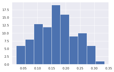
Because it holds the raw data of the total causal effect (the original data for calculating the median), it is possible to draw a histogram of the values of the causal effect, as shown below.
import matplotlib.pyplot as plt
import seaborn as sns
sns.set()
%matplotlib inline

from_index = 5 # index of x0(1). (index:0)+(n_features:5)*(timepoint:1) = 5
to_index = 12 # index of x2(2). (index:2)+(n_features:5)*(timepoint:2) = 12
plt.hist(result.total_effects_[:, to_index, from_index])