RCD
Model
This method RCD (Repetitive Causal Discovery) [3] assumes an extension of the basic LiNGAM model [1] to hidden common cause cases, i.e., the latent variable LiNGAM model [2]. Similarly to the basic LiNGAM model [1], this method makes the following assumptions:
Linearity
Non-Gaussian continuous error variables
Acyclicity
However, RCD allows the existence of hidden common causes. It outputs a causal graph where a bi-directed arc indicates the pair of variables that have the same hidden common causes, and a directed arrow indicates the causal direction of a pair of variables that are not affected by the same hidden common causes.
References
Import and settings
In this example, we need to import numpy, pandas, and
graphviz in addition to lingam.
import numpy as np
import pandas as pd
import graphviz
import lingam
from lingam.utils import print_causal_directions, print_dagc, make_dot

print([np.__version__, pd.__version__, graphviz.__version__, lingam.__version__])

np.set_printoptions(precision=3, suppress=True)
['1.24.4', '2.0.3', '0.20.1', '1.8.3']
Test data
First, we generate a causal structure with 7 variables. Then we create a dataset with 5 variables from x0 to x4, with x5 and x6 being the latent variables.
np.random.seed(0)

get_external_effect = lambda n: np.random.normal(0.0, 0.5, n) ** 3
n_samples = 300

x5 = get_external_effect(n_samples)
x6 = get_external_effect(n_samples)
x1 = 0.6*x5 + get_external_effect(n_samples)
x3 = 0.5*x5 + get_external_effect(n_samples)
x0 = 1.0*x1 + 1.0*x3 + get_external_effect(n_samples)
x2 = 0.8*x0 - 0.6*x6 + get_external_effect(n_samples)
x4 = 1.0*x0 - 0.5*x6 + get_external_effect(n_samples)

# The latent variable x6 is not included.
X = pd.DataFrame(np.array([x0, x1, x2, x3, x4, x5]).T, columns=['x0', 'x1', 'x2', 'x3', 'x4', 'x5'])

X.head()
| x0 | x1 | x2 | x3 | x4 | x5 | |
|---|---|---|---|---|---|---|
| 0 | -0.191493 | -0.054157 | 0.014075 | -0.047309 | 0.016311 | 0.686190 |
| 1 | -0.967142 | 0.013890 | -1.115854 | -0.035899 | -1.254783 | 0.008009 |
| 2 | 0.527409 | -0.034960 | 0.426923 | 0.064804 | 0.894242 | 0.117195 |
| 3 | 1.583826 | 0.845653 | 1.265038 | 0.704166 | 1.994283 | 1.406609 |
| 4 | 0.286276 | 0.141120 | 0.116967 | 0.329866 | 0.257932 | 0.814202 |
m = np.array([[ 0.0, 1.0, 0.0, 1.0, 0.0, 0.0, 0.0],
              [ 0.0, 0.0, 0.0, 0.0, 0.0, 0.6, 0.0],
              [ 0.8, 0.0, 0.0, 0.0, 0.0, 0.0,-0.6],
              [ 0.0, 0.0, 0.0, 0.0, 0.0, 0.5, 0.0],
              [ 1.0, 0.0, 0.0, 0.0, 0.0, 0.0,-0.5],
              [ 0.0, 0.0, 0.0, 0.0, 0.0, 0.0, 0.0],
              [ 0.0, 0.0, 0.0, 0.0, 0.0, 0.0, 0.0]])
dot = make_dot(m, labels=['x0', 'x1', 'x2', 'x3', 'x4', 'x5', 'f1(x6)'])

# Save pdf
dot.render('dag')

# Save png
dot.format = 'png'
dot.render('dag')

dot

Causal Discovery
To run causal discovery, we create a RCD object and call the fit
method.
model = lingam.RCD()
model.fit(X)
<lingam.rcd.RCD at 0x7f76b338e8b0>
Using the ancestors_list_ properties, we can see the list of
ancestors sets as a result of the causal discovery.
ancestors_list = model.ancestors_list_

for i, ancestors in enumerate(ancestors_list):
    print(f'M{i}={ancestors}')
M0={1, 3, 5}
M1={5}
M2={0, 1, 3, 5}
M3={5}
M4={0, 1, 3, 5}
M5=set()
Also, using the adjacency_matrix_ properties, we can see the
adjacency matrix as a result of the causal discovery. The coefficients
between variables with latent confounders are np.nan.
model.adjacency_matrix_
array([[0.   , 0.939, 0.   , 0.994, 0.   , 0.   ],
       [0.   , 0.   , 0.   , 0.   , 0.   , 0.556],
       [0.751, 0.   , 0.   , 0.   ,   nan, 0.   ],
       [0.   , 0.   , 0.   , 0.   , 0.   , 0.563],
       [1.016, 0.   ,   nan, 0.   , 0.   , 0.   ],
       [0.   , 0.   , 0.   , 0.   , 0.   , 0.   ]])
make_dot(model.adjacency_matrix_)

Independence between error variables
To check if the LiNGAM assumption is broken, we can get p-values of independence between error variables. The value in the i-th row and j-th column of the obtained matrix shows the p-value of the independence of the error variables \(e_i\) and \(e_j\).
p_values = model.get_error_independence_p_values(X)
print(p_values)
[[0.    0.      nan 0.413   nan 0.68 ]
 [0.    0.      nan 0.732   nan 0.382]
 [  nan   nan 0.      nan   nan   nan]
 [0.413 0.732   nan 0.      nan 0.054]
 [  nan   nan   nan   nan 0.      nan]
 [0.68  0.382   nan 0.054   nan 0.   ]]
Bootstrapping
We call bootstrap() method instead of fit(). Here, the second
argument specifies the number of bootstrap sampling.
import warnings
warnings.filterwarnings('ignore', category=UserWarning)

model = lingam.RCD()
result = model.bootstrap(X, n_sampling=100)
Causal Directions
Since BootstrapResult object is returned, we can get the ranking of
the causal directions extracted by get_causal_direction_counts()
method. In the following sample code, n_directions option is limited
to the causal directions of the top 8 rankings, and
min_causal_effect option is limited to causal directions with a
coefficient of 0.01 or more.
cdc = result.get_causal_direction_counts(n_directions=8, min_causal_effect=0.01, split_by_causal_effect_sign=True)
We can check the result by utility function.
print_causal_directions(cdc, 100)
x4 <--- x0 (b>0) (58.0%)
x0 <--- x5 (b>0) (51.0%)
x2 <--- x0 (b>0) (30.0%)
x3 <--- x5 (b>0) (30.0%)
x0 <--- x1 (b>0) (22.0%)
x0 <--- x3 (b>0) (18.0%)
x1 <--- x5 (b>0) (18.0%)
x2 <--- x5 (b>0) (15.0%)
Directed Acyclic Graphs
Also, using the get_directed_acyclic_graph_counts() method, we can
get the ranking of the DAGs extracted. In the following sample code,
n_dags option is limited to the dags of the top 3 rankings, and
min_causal_effect option is limited to causal directions with a
coefficient of 0.01 or more.
dagc = result.get_directed_acyclic_graph_counts(n_dags=3, min_causal_effect=0.01, split_by_causal_effect_sign=True)
We can check the result by utility function.
print_dagc(dagc, 100)
DAG[0]: 6.0%
DAG[1]: 4.0%
    x4 <--- x0 (b>0)
DAG[2]: 4.0%
    x2 <--- x0 (b>0)
Probability
Using the get_probabilities() method, we can get the probability of
bootstrapping.
prob = result.get_probabilities(min_causal_effect=0.01)
print(prob)
[[0.   0.22 0.   0.18 0.   0.51]
 [0.   0.   0.   0.   0.   0.18]
 [0.3  0.13 0.   0.12 0.05 0.15]
 [0.   0.   0.   0.   0.   0.3 ]
 [0.58 0.11 0.02 0.11 0.   0.05]
 [0.   0.   0.   0.   0.   0.  ]]
Total Causal Effects
Using the get_total_causal_effects() method, we can get the list of
total causal effect. The total causal effects we can get are dictionary
type variable. We can display the list nicely by assigning it to
pandas.DataFrame. Also, we have replaced the variable index with a label
below.
causal_effects = result.get_total_causal_effects(min_causal_effect=0.01)

# Assign to pandas.DataFrame for pretty display
df = pd.DataFrame(causal_effects)
labels = [f'x{i}' for i in range(X.shape[1])]
df['from'] = df['from'].apply(lambda x : labels[x])
df['to'] = df['to'].apply(lambda x : labels[x])
df
| from | to | effect | probability | |
|---|---|---|---|---|
| 0 | x3 | x0 | 1.055784 | 0.04 |
| 1 | x3 | x2 | 0.818606 | 0.04 |
| 2 | x4 | x2 | 0.484138 | 0.04 |
| 3 | x3 | x4 | 1.016508 | 0.04 |
| 4 | x1 | x0 | 0.929668 | 0.03 |
| 5 | x0 | x2 | 0.781983 | 0.03 |
| 6 | x0 | x4 | 1.003733 | 0.03 |
| 7 | x1 | x4 | 1.041410 | 0.03 |
| 8 | x1 | x2 | 0.730836 | 0.02 |
| 9 | x5 | x0 | 0.961161 | 0.01 |
| 10 | x5 | x1 | 0.542628 | 0.01 |
| 11 | x5 | x3 | 0.559532 | 0.01 |
We can easily perform sorting operations with pandas.DataFrame.
df.sort_values('effect', ascending=False).head()
| from | to | effect | probability | |
|---|---|---|---|---|
| 0 | x3 | x0 | 1.055784 | 0.04 |
| 7 | x1 | x4 | 1.041410 | 0.03 |
| 3 | x3 | x4 | 1.016508 | 0.04 |
| 6 | x0 | x4 | 1.003733 | 0.03 |
| 9 | x5 | x0 | 0.961161 | 0.01 |
df.sort_values('probability', ascending=True).head()
| from | to | effect | probability | |
|---|---|---|---|---|
| 9 | x5 | x0 | 0.961161 | 0.01 |
| 10 | x5 | x1 | 0.542628 | 0.01 |
| 11 | x5 | x3 | 0.559532 | 0.01 |
| 8 | x1 | x2 | 0.730836 | 0.02 |
| 4 | x1 | x0 | 0.929668 | 0.03 |
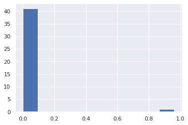
Because it holds the raw data of the causal effect (the original data for calculating the median), it is possible to draw a histogram of the values of the causal effect, as shown below.
import matplotlib.pyplot as plt
import seaborn as sns
sns.set()
%matplotlib inline

from_index = 5 # index of x5
to_index = 0 # index of x0
plt.hist(result.total_effects_[:, to_index, from_index])
Bootstrap Probability of Path
Using the get_paths() method, we can explore all paths from any
variable to any variable and calculate the bootstrap probability for
each path. The path will be output as an array of variable indices. For
example, the array [3, 0, 1] shows the path from variable X3 through
variable X0 to variable X1.
from_index = 5 # index of x5
to_index = 4 # index of x4

pd.DataFrame(result.get_paths(from_index, to_index))
| path | effect | probability | |
|---|---|---|---|
| 0 | [5, 0, 4] | 0.970828 | 0.34 |
| 1 | [5, 3, 0, 4] | 0.522827 | 0.07 |
| 2 | [5, 3, 4] | 0.461104 | 0.06 |
| 3 | [5, 4] | 0.821702 | 0.05 |
| 4 | [5, 1, 0, 4] | 0.605828 | 0.02 |
| 5 | [5, 1, 4] | 0.574573 | 0.02 |