BottomUpParceLiNGAM
Model
This method assumes an extension of the basic LiNGAM model [1] to hidden common cause cases. Specifically, this implements Algorithm 1 of [3] except the Step 2. Similarly to the basic LiNGAM model [1], this method makes the following assumptions:
Linearity
Non-Gaussian continuous error variables (except at most one)
Acyclicity
However, it allows the following hidden common causes:
Only exogenous observed variables may share hidden common causes.
This is a simpler version of the latent variable LiNGAM [2] that extends the basic LiNGAM model to hidden common causes. Note that the latent variable LiNGAM [2] allows the existence of hidden common causes between any observed variables. However, this kind of causal graph structures are often assumed in the classic structural equation modelling [4].
Denote observed variables by \({x}_{i}\) and error variables by \({e}_{i}\) and coefficients or connection strengths \({b}_{ij}\). Collect them in vectors \({x}\) and \({e}\) and a matrix \({B}\), respectivelly. Due to the acyclicity assumption, the adjacency matrix \({B}\) can be permuted to be strictly lower-triangular by a simultaneous row and column permutation. The error variables \({e}_{i}\) except those corresponding to exogenous observed variables are independent due to the assumption that only exogenous observed variables may share hidden common causes.
Then, mathematically, the model for observed variable vector \({x}\) is written as
$$ x = Bx + e. $$
References
Import and settings
In this example, we need to import numpy, pandas, and
graphviz in addition to lingam.
import numpy as np
import pandas as pd
import graphviz
import lingam
from lingam.utils import print_causal_directions, print_dagc, make_dot

import warnings
warnings.filterwarnings('ignore')

print([np.__version__, pd.__version__, graphviz.__version__, lingam.__version__])

np.set_printoptions(precision=3, suppress=True)
['1.24.4', '2.0.3', '0.20.1', '1.8.3']
Test data
First, we generate a causal structure with 7 variables. Then we create a dataset with 6 variables from x0 to x5, with x6 being the latent variable for x2 and x3.
np.random.seed(1000)

x6 = np.random.uniform(size=1000)
x3 = 2.0*x6 + np.random.uniform(size=1000)
x0 = 0.5*x3 + np.random.uniform(size=1000)
x2 = 2.0*x6 + np.random.uniform(size=1000)
x1 = 0.5*x0 + 0.5*x2 + np.random.uniform(size=1000)
x5 = 0.5*x0 + np.random.uniform(size=1000)
x4 = 0.5*x0 - 0.5*x2 + np.random.uniform(size=1000)

# The latent variable x6 is not included.
X = pd.DataFrame(np.array([x0, x1, x2, x3, x4, x5]).T, columns=['x0', 'x1', 'x2', 'x3', 'x4', 'x5'])

X.head()
| x0 | x1 | x2 | x3 | x4 | x5 | |
|---|---|---|---|---|---|---|
| 0 | 1.505949 | 2.667827 | 2.029420 | 1.463708 | 0.615387 | 1.157907 |
| 1 | 1.379130 | 1.721744 | 0.965613 | 0.801952 | 0.919654 | 0.957148 |
| 2 | 1.436825 | 2.845166 | 2.773506 | 2.533417 | -0.616746 | 0.903326 |
| 3 | 1.562885 | 2.205270 | 1.080121 | 1.192257 | 1.240595 | 1.411295 |
| 4 | 1.940721 | 2.974182 | 2.140298 | 1.886342 | 0.451992 | 1.770786 |
m = np.array([[0.0, 0.0, 0.0, 0.5, 0.0, 0.0, 0.0],
              [0.5, 0.0, 0.5, 0.0, 0.0, 0.0, 0.0],
              [0.0, 0.0, 0.0, 0.0, 0.0, 0.0, 2.0],
              [0.0, 0.0, 0.0, 0.0, 0.0, 0.0, 2.0],
              [0.5, 0.0,-0.5, 0.0, 0.0, 0.0, 0.0],
              [0.5, 0.0, 0.0, 0.0, 0.0, 0.0, 0.0],
              [0.0, 0.0, 0.0, 0.0, 0.0, 0.0, 0.0]])

dot = make_dot(m)

# Save pdf
dot.render('dag')

# Save png
dot.format = 'png'
dot.render('dag')

dot

Causal Discovery
To run causal discovery, we create a BottomUpParceLiNGAM object and
call the fit method.
model = lingam.BottomUpParceLiNGAM()
model.fit(X)
<lingam.bottom_up_parce_lingam.BottomUpParceLiNGAM at 0x7fb69052ca60>
Using the causal_order_ properties, we can see the causal ordering
as a result of the causal discovery. x2 and x3, which have latent
confounders as parents, are stored in a list without causal ordering.
model.causal_order_
[[2, 3], 0, 5, 1, 4]
Also, using the adjacency_matrix_ properties, we can see the
adjacency matrix as a result of the causal discovery. The coefficients
between variables with latent confounders are np.nan.
model.adjacency_matrix_
array([[ 0.   ,  0.   ,  0.   ,  0.511,  0.   ,  0.   ],
       [ 0.504,  0.   ,  0.499,  0.   ,  0.   ,  0.   ],
       [ 0.   ,  0.   ,  0.   ,    nan,  0.   ,  0.   ],
       [ 0.   ,  0.   ,    nan,  0.   ,  0.   ,  0.   ],
       [ 0.481,  0.   , -0.473,  0.   ,  0.   ,  0.   ],
       [ 0.519,  0.   ,  0.   ,  0.   ,  0.   ,  0.   ]])
We can draw a causal graph by utility funciton.
make_dot(model.adjacency_matrix_)

Independence between error variables
To check if the LiNGAM assumption is broken, we can get p-values of independence between error variables. The value in the i-th row and j-th column of the obtained matrix shows the p-value of the independence of the error variables \(e_i\) and \(e_j\).
p_values = model.get_error_independence_p_values(X)
print(p_values)
[[0.    0.523   nan   nan 0.8   0.399]
 [0.523 0.      nan   nan 0.44  0.6  ]
 [  nan   nan 0.      nan   nan   nan]
 [  nan   nan   nan 0.      nan   nan]
 [0.8   0.44    nan   nan 0.    0.446]
 [0.399 0.6     nan   nan 0.446 0.   ]]
Bootstrapping
We call bootstrap() method instead of fit(). Here, the second
argument specifies the number of bootstrap sampling.
import warnings
warnings.filterwarnings('ignore', category=UserWarning)

model = lingam.BottomUpParceLiNGAM()
result = model.bootstrap(X, n_sampling=100)
Causal Directions
Since BootstrapResult object is returned, we can get the ranking of
the causal directions extracted by get_causal_direction_counts()
method. In the following sample code, n_directions option is limited
to the causal directions of the top 8 rankings, and
min_causal_effect option is limited to causal directions with a
coefficient of 0.01 or more.
cdc = result.get_causal_direction_counts(n_directions=8, min_causal_effect=0.01, split_by_causal_effect_sign=True)
We can check the result by utility function.
print_causal_directions(cdc, 100)
x4 <--- x0 (b>0) (45.0%)
x4 <--- x2 (b<0) (45.0%)
x1 <--- x0 (b>0) (41.0%)
x1 <--- x2 (b>0) (41.0%)
x5 <--- x0 (b>0) (26.0%)
x0 <--- x3 (b>0) (12.0%)
x1 <--- x4 (b>0) (6.0%)
x4 <--- x1 (b>0) (4.0%)
Directed Acyclic Graphs
Also, using the get_directed_acyclic_graph_counts() method, we can
get the ranking of the DAGs extracted. In the following sample code,
n_dags option is limited to the dags of the top 3 rankings, and
min_causal_effect option is limited to causal directions with a
coefficient of 0.01 or more.
dagc = result.get_directed_acyclic_graph_counts(n_dags=3, min_causal_effect=0.01, split_by_causal_effect_sign=True)
We can check the result by utility function.
print_dagc(dagc, 100)
DAG[0]: 33.0%
DAG[1]: 12.0%
    x4 <--- x0 (b>0)
    x4 <--- x2 (b<0)
DAG[2]: 10.0%
    x0 <--- x3 (b>0)
    x1 <--- x0 (b>0)
    x1 <--- x2 (b>0)
    x4 <--- x0 (b>0)
    x4 <--- x2 (b<0)
    x5 <--- x0 (b>0)
Probability
Using the get_probabilities() method, we can get the probability of
bootstrapping.
prob = result.get_probabilities(min_causal_effect=0.01)
print(prob)
[[0.   0.01 0.   0.12 0.01 0.  ]
 [0.41 0.   0.41 0.   0.06 0.  ]
 [0.   0.   0.   0.02 0.   0.  ]
 [0.   0.   0.   0.   0.   0.  ]
 [0.45 0.04 0.45 0.02 0.   0.01]
 [0.26 0.   0.   0.   0.   0.  ]]
Total Causal Effects
Using the get_total_causal_effects() method, we can get the list of
total causal effect. The total causal effects we can get are dictionary
type variable. We can display the list nicely by assigning it to
pandas.DataFrame. Also, we have replaced the variable index with a label
below.
causal_effects = result.get_total_causal_effects(min_causal_effect=0.01)

# Assign to pandas.DataFrame for pretty display
df = pd.DataFrame(causal_effects)
labels = [f'x{i}' for i in range(X.shape[1])]
df['from'] = df['from'].apply(lambda x : labels[x])
df['to'] = df['to'].apply(lambda x : labels[x])
df
| from | to | effect | probability | |
|---|---|---|---|---|
| 0 | x0 | x5 | 0.518064 | 0.12 |
| 1 | x0 | x1 | 0.504613 | 0.11 |
| 2 | x0 | x4 | 0.479543 | 0.11 |
| 3 | x2 | x1 | 0.508531 | 0.02 |
| 4 | x2 | x4 | -0.476555 | 0.02 |
| 5 | x3 | x0 | 0.490217 | 0.01 |
| 6 | x3 | x1 | 0.630292 | 0.01 |
| 7 | x4 | x1 | 0.097063 | 0.01 |
| 8 | x3 | x2 | 0.796101 | 0.01 |
| 9 | x1 | x4 | 0.089596 | 0.01 |
| 10 | x3 | x4 | -0.151733 | 0.01 |
| 11 | x3 | x5 | 0.254280 | 0.01 |
We can easily perform sorting operations with pandas.DataFrame.
df.sort_values('effect', ascending=False).head()
| from | to | effect | probability | |
|---|---|---|---|---|
| 8 | x3 | x2 | 0.796101 | 0.01 |
| 6 | x3 | x1 | 0.630292 | 0.01 |
| 0 | x0 | x5 | 0.518064 | 0.12 |
| 3 | x2 | x1 | 0.508531 | 0.02 |
| 1 | x0 | x1 | 0.504613 | 0.11 |
df.sort_values('probability', ascending=True).head()
| from | to | effect | probability | |
|---|---|---|---|---|
| 5 | x3 | x0 | 0.490217 | 0.01 |
| 6 | x3 | x1 | 0.630292 | 0.01 |
| 7 | x4 | x1 | 0.097063 | 0.01 |
| 8 | x3 | x2 | 0.796101 | 0.01 |
| 9 | x1 | x4 | 0.089596 | 0.01 |
And with pandas.DataFrame, we can easily filter by keywords. The following code extracts the causal direction towards x1.
df[df['to']=='x1'].head()
| from | to | effect | probability | |
|---|---|---|---|---|
| 1 | x0 | x1 | 0.504613 | 0.11 |
| 3 | x2 | x1 | 0.508531 | 0.02 |
| 6 | x3 | x1 | 0.630292 | 0.01 |
| 7 | x4 | x1 | 0.097063 | 0.01 |
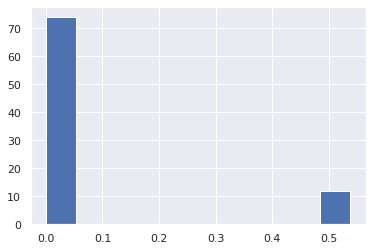
Because it holds the raw data of the total causal effect (the original data for calculating the median), it is possible to draw a histogram of the values of the causal effect, as shown below.
import matplotlib.pyplot as plt
import seaborn as sns
sns.set()
%matplotlib inline

from_index = 0 # index of x0
to_index = 5 # index of x5
plt.hist(result.total_effects_[:, to_index, from_index])
Bootstrap Probability of Path
Using the get_paths() method, we can explore all paths from any
variable to any variable and calculate the bootstrap probability for
each path. The path will be output as an array of variable indices. For
example, the array [3, 0, 1] shows the path from variable X3 through
variable X0 to variable X1.
from_index = 3 # index of x3
to_index = 1 # index of x0

pd.DataFrame(result.get_paths(from_index, to_index))
| path | effect | probability | |
|---|---|---|---|
| 0 | [3, 0, 1] | 0.263068 | 0.11 |
| 1 | [3, 2, 1] | 0.404828 | 0.02 |